Mosaic Integration of RNA+ADT+ATAC#
In this tutorial, we demonstrate how to integrate a mosaic dataset consisting of RNA, ADT, and ATAC data. We will also walk through the inference process and the outputs generated by MIDAS.
Step 1: Downloading the Demo Data#
[ ]:
from scmidas.data import download_data
download_data('teadog_mosaic_4k', './dataset')
Step 2: Setting Up the Environment#
Before we begin, ensure that the required environment is set up. This includes importing the necessary packages and dependencies.
[ ]:
import os
os.environ['CUDA_VISIBLE_DEVICES']='0'

from scmidas.config import load_config
from scmidas.model import MIDAS
from scmidas.utils import load_predicted
import lightning as L

import pandas as pd
import numpy as np
import scanpy as sc
import matplotlib.pyplot as plt
from scipy.stats import pearsonr
from sklearn.metrics import roc_auc_score

sc.set_figure_params(figsize=(4, 4))
Step 3: Configuring the Model#
In this step, we configure the model for our dataset. Since we define the ATAC data as a Bernoulli distribution, we first binarize the data before modeling it with MIDAS.
[ ]:
configs = load_config()
[ ]:
task = 'teadog_mosaic_4k'
transfrom = {'atac':'binarize'}
model = MIDAS.configure_data_from_dir(configs, './dataset/'+task+'/data', transfrom)
INFO:root:Input data:
         #CELL    #ATAC    #RNA   #ADT  #VALID_RNA  #VALID_ADT
BATCH 0   1000  31243.0  4047.0    NaN      3809.0         NaN
BATCH 1   1000  31243.0     NaN  213.0         NaN        45.0
BATCH 2   1000      NaN  4047.0  213.0      3862.0       208.0
BATCH 3   1000  31243.0  4047.0  213.0      3751.0       208.0
Step 4: Training the Model (~2h)#
After configuring the model, we proceed with training. This step typically takes around 2 hours using a single V100 GPU, depending on your system’s specifications. If you prefer a quicker result, you can set max_epochs=500 for a reasonable outcome, instead of the default max_epochs=2000 for the best result.
[ ]:
trainer = L.Trainer(
    accelerator='auto',
    devices=1,
    precision=32,
    strategy='auto',
    num_nodes=1,
    max_epochs=2000,
    log_every_n_steps= 5)
trainer.fit(model=model)
GPU available: True (cuda), used: True
TPU available: False, using: 0 TPU cores
HPU available: False, using: 0 HPUs
LOCAL_RANK: 0 - CUDA_VISIBLE_DEVICES: [0]

  | Name | Type          | Params | Mode
-----------------------------------------------
0 | net  | VAE           | 49.8 M | train
1 | dsc  | Discriminator | 52.3 K | train
-----------------------------------------------
49.8 M    Trainable params
0         Non-trainable params
49.8 M    Total params
199.357   Total estimated model params size (MB)
676       Modules in train mode
0         Modules in eval mode
INFO:root:Total number of samples: 4000 from 4 datasets.
INFO:root:Using MultiBatchSampler for data loading.
/root/anaconda3/envs/pl/lib/python3.12/site-packages/torch/utils/data/sampler.py:76: UserWarning: `data_source` argument is not used and will be removed in 2.2.0.You may still have custom implementation that utilizes it.
  warnings.warn(
INFO:root:DataLoader created with batch size 256 and 20 workers.
Epoch 500: 100%|██████████| 16/16 [00:04<00:00, 3.39it/s, v_num=c_4k, loss_/recon_loss_step=3.06e+3, loss_/kld_loss_step=113.0, loss_/consistency_loss_step=30.70, loss/net_step=3.11e+3, loss/dsc_step=97.10, loss_/recon_loss_epoch=9.27e+3, loss_/kld_loss_epoch=116.0, loss_/consistency_loss_epoch=33.50, loss/net_epoch=9.32e+3, loss/dsc_epoch=105.0]
INFO:root:Checkpoint successfully saved to "./saved_models/model_epoch500_20241212-032436.pt".
INFO:root:Checkpoint saved for epoch "500" at "./saved_models/model_epoch500_20241212-032436.pt".
Epoch 1000: 100%|██████████| 16/16 [00:04<00:00, 3.79it/s, v_num=c_4k, loss_/recon_loss_step=8.26e+3, loss_/kld_loss_step=111.0, loss_/consistency_loss_step=28.90, loss/net_step=8.29e+3, loss/dsc_step=103.0, loss_/recon_loss_epoch=8.9e+3, loss_/kld_loss_epoch=121.0, loss_/consistency_loss_epoch=24.70, loss/net_epoch=8.94e+3, loss/dsc_epoch=106.0]
INFO:root:Checkpoint successfully saved to "./saved_models/model_epoch1000_20241212-040104.pt".
INFO:root:Checkpoint saved for epoch "1000" at "./saved_models/model_epoch1000_20241212-040104.pt".
Epoch 1500: 100%|██████████| 16/16 [00:04<00:00, 3.69it/s, v_num=c_4k, loss_/recon_loss_step=2.98e+3, loss_/kld_loss_step=116.0, loss_/consistency_loss_step=23.10, loss/net_step=3.02e+3, loss/dsc_step=98.80, loss_/recon_loss_epoch=8.69e+3, loss_/kld_loss_epoch=124.0, loss_/consistency_loss_epoch=23.40, loss/net_epoch=8.73e+3, loss/dsc_epoch=105.0]
INFO:root:Checkpoint successfully saved to "./saved_models/model_epoch1500_20241212-044030.pt".
INFO:root:Checkpoint saved for epoch "1500" at "./saved_models/model_epoch1500_20241212-044030.pt".
Epoch 1999: 100%|██████████| 16/16 [00:04<00:00, 3.35it/s, v_num=c_4k, loss_/recon_loss_step=1.2e+4, loss_/kld_loss_step=135.0, loss_/consistency_loss_step=38.40, loss/net_step=1.2e+4, loss/dsc_step=129.0, loss_/recon_loss_epoch=8.52e+3, loss_/kld_loss_epoch=125.0, loss_/consistency_loss_epoch=23.10, loss/net_epoch=8.56e+3, loss/dsc_epoch=104.0]
`Trainer.fit` stopped: `max_epochs=2000` reached.
Epoch 1999: 100%|██████████| 16/16 [00:04<00:00, 3.34it/s, v_num=c_4k, loss_/recon_loss_step=1.2e+4, loss_/kld_loss_step=135.0, loss_/consistency_loss_step=38.40, loss/net_step=1.2e+4, loss/dsc_step=129.0, loss_/recon_loss_epoch=8.52e+3, loss_/kld_loss_epoch=125.0, loss_/consistency_loss_epoch=23.10, loss/net_epoch=8.56e+3, loss/dsc_epoch=104.0]
INFO:root:Checkpoint successfully saved to "./saved_models/model_epoch2000_20241212-051907.pt".
INFO:root:Checkpoint saved for epoch "2000" at ./saved_models/model_epoch2000_20241212-051907.pt".
Step 5: Predicting#
Once the model is trained, we can run predict() to obtain various outputs from MIDAS.
[ ]:
# load a checkpoint
# model.load_checkpoint('./saved_models/model_epoch2000_20241212-051907.pt')
[ ]:
model.predict('./predict/'+task,
        joint_latent=True,
        mod_latent=True,
        impute=True,
        batch_correct=True,
        translate=True,
        input=True)
Outputs: Joint Embeddings#
In this step, we explore the various outputs generated by MIDAS. First, we load the labels associated with the dataset.
[ ]:
label = []
batch_id = []
for i in ['w1', 'w6', 'lll_ctrl', 'dig_stim']:
    label.append(pd.read_csv('./dataset/'+task+'/label/%s.csv'%i, index_col=0).values.flatten()[:1000])
    batch_id.append([i] * 1000)
labels = np.concatenate(label)
batch_ids = np.concatenate(batch_id)
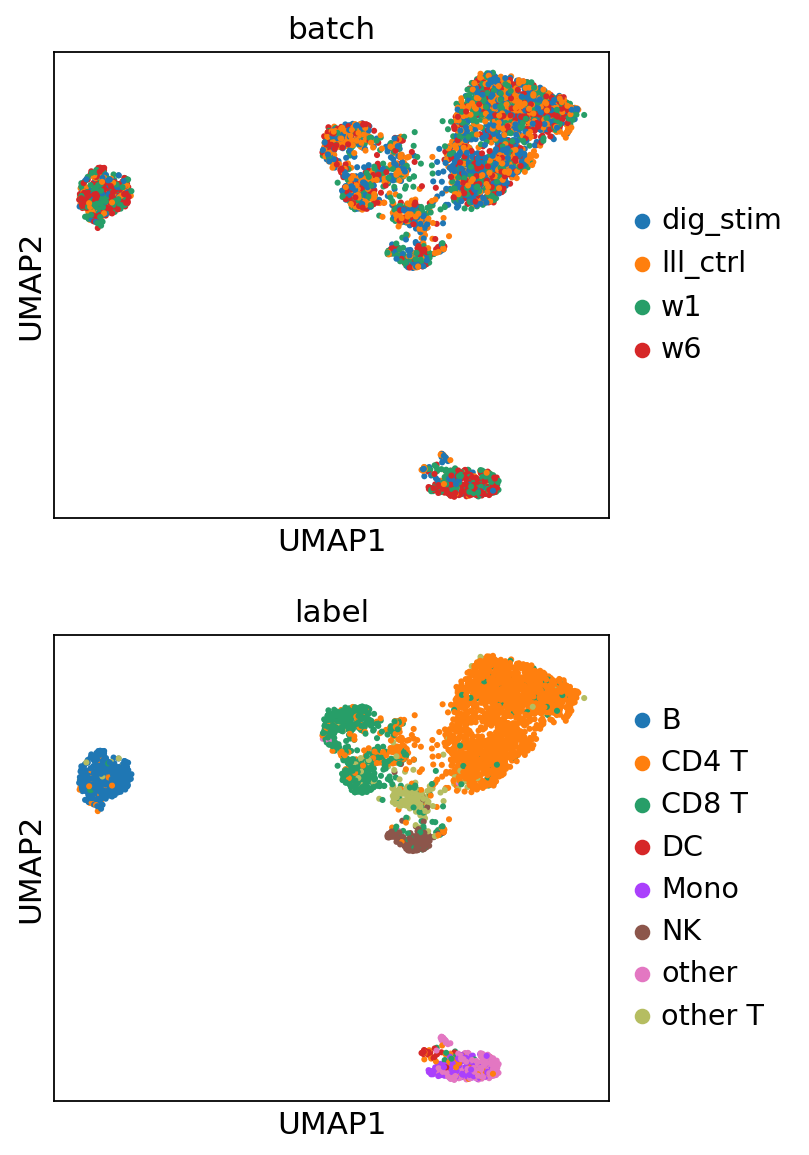
The joint embeddings consist of two components: biological information (c) and technical information (u). To analyze them, we split the embeddings and visualize them separately.
[ ]:
joint_embeddings = load_predicted('./predict/'+task, model.combs, joint_latent=True)

adata_bio = sc.AnnData(joint_embeddings['z']['joint'][:, :model.dim_c])
adata_tech = sc.AnnData(joint_embeddings['z']['joint'][:, model.dim_c:])

adata_bio.obs['batch'] = batch_ids
adata_bio.obs['label'] = labels
adata_tech.obs['batch'] = batch_ids
adata_tech.obs['label'] = labels

for adata in [adata_bio, adata_tech]:
    sc.pp.neighbors(adata)
    sc.tl.umap(adata)
    #shuffle
    sc.pp.subsample(adata, fraction=1)
    sc.pl.umap(adata, color=['batch', 'label'], ncols=2)
INFO:root:Loading predicted variables ...
INFO:root:Loading batch 0: z, joint
100%|██████████| 4/4 [00:00<00:00, 154.06it/s]
INFO:root:Loading batch 1: z, joint
100%|██████████| 4/4 [00:00<00:00, 150.67it/s]
INFO:root:Loading batch 2: z, joint
100%|██████████| 4/4 [00:00<00:00, 157.83it/s]
INFO:root:Loading batch 3: z, joint
100%|██████████| 4/4 [00:00<00:00, 147.54it/s]
INFO:root:Converting to numpy ...
INFO:root:Converting batch 0: s, joint
INFO:root:Converting batch 0: z, joint
INFO:root:Converting batch 1: s, joint
INFO:root:Converting batch 1: z, joint
INFO:root:Converting batch 2: s, joint
INFO:root:Converting batch 2: z, joint
INFO:root:Converting batch 3: s, joint
INFO:root:Converting batch 3: z, joint
/root/anaconda3/envs/pl/lib/python3.12/site-packages/tqdm/auto.py:21: TqdmWarning: IProgress not found. Please update jupyter and ipywidgets. See https://ipywidgets.readthedocs.io/en/stable/user_install.html
  from .autonotebook import tqdm as notebook_tqdm
... storing 'batch' as categorical
... storing 'label' as categorical

... storing 'batch' as categorical
... storing 'label' as categorical
Outputs: Modality-specific Embeddings#
Here, we check the alignment among modalities by visualizing them with UMAP.
[ ]:
mod_embeddings = load_predicted('./predict/'+task, model.combs, mod_latent=True, group_by='batch')
batch_names = ['w1', 'w6', 'lll_ctrl', 'dig_stim']
adata_list = []
for i in range(model.dims_s['joint']):
    for m in model.mods+['joint']:
        if m in mod_embeddings[i]['z']:
            adata = sc.AnnData(mod_embeddings[i]['z'][m][:, :model.dim_c])
            adata.obs['batch'] = batch_names[i]
            adata.obs['modality'] = m
            adata.obs['label'] = label[i]
            adata_list.append(adata)
adata_mod_concat = sc.concat(adata_list)
for i in adata_mod_concat.obs:
    adata_mod_concat.obs[i] = adata_mod_concat.obs[i].astype('category')
sc.pp.neighbors(adata_mod_concat)
# shuffle
sc.pp.subsample(adata_mod_concat, fraction=1)
sc.tl.umap(adata_mod_concat)
[10]:
# setup figure
nrows = len(model.mods) + 1
ncols = model.dims_s['joint']
point_size = 20

fig, ax = plt.subplots(nrows, ncols, figsize=[2 * ncols, 2 * nrows])

# set up the name of modalities and batch
mod_names = model.mods + ['joint']

# iteratively scatter the data
for i, mod in enumerate(mod_names):
    for b in range(model.dims_s['joint']):
        # filter data
        adata = adata_mod_concat[
            (adata_mod_concat.obs['modality'] == mod) &
            (adata_mod_concat.obs['batch'] == batch_names[b])
        ].copy()
        if len(adata):
            sc.pl.umap(adata, color='label', show=False, ax=ax[i, b], s=point_size)
            ax[i, b].get_legend().set_visible(False)
            handles, labels_ = ax[i, b].get_legend_handles_labels()
        ax[i, b].set_xticks([])
        ax[i, b].set_yticks([])
        ax[i, b].set_xlabel('')
        if b==0:
            ax[i, b].set_ylabel(mod.upper())
        else:
            ax[i, b].set_ylabel('')
        if i==0:
            ax[i, b].set_title(batch_names[b])
        else:
            ax[i, b].set_title('')
# create global legend
fig.legend(handles, labels_, loc='center', bbox_to_anchor=(0.5, -0.02), ncol=len(labels_), fontsize=10)

# adjust the figure
plt.tight_layout(rect=[0.1, 0.05, 1, 1])
plt.show()

Outputs: Imputed Counts#
Here, we retrieve the imputed ADT from batch 0, RNA from batch 1, and ATAC from batch 2. Then we calculate the similarity between the predicted counts and the ground-truth counts.
[ ]:
imputed = load_predicted('./predict/'+task, model.combs, impute=True)
[ ]:
ref_adt = pd.read_csv('./dataset/'+task+'/data/batch_0/mat/adt.csv', index_col=0).iloc[:1000].values
print('Pearson\'s r for ADT (BATCH 0)', pearsonr(ref_adt.reshape(-1), imputed['x_impt']['adt'][:1000].reshape(-1))[0])
Pearson's r for ADT (BATCH 0) 0.4553754578268669
[ ]:
ref_adt = pd.read_csv('./dataset/'+task+'/data/batch_1/mat/rna.csv', index_col=0).iloc[:1000].values
print('Pearson\'s r for RNA (BATCH 1)', pearsonr(ref_adt.reshape(-1), imputed['x_impt']['rna'][1000:2000].reshape(-1))[0])
Pearson's r for RNA (BATCH 1) 0.5388385375124954
[ ]:
ref_atac = pd.read_csv('./dataset/'+task+'/data/batch_2/mat/atac.csv', index_col=0).iloc[:1000].values.reshape(-1)
ref_atac = np.where(ref_atac>0.5, 1, 0) #binarize
print('AUROC for ATAC (BATCH 2)', roc_auc_score(ref_atac, imputed['x_impt']['atac'][2000:3000].reshape(-1)))
AUROC for ATAC (BATCH 2) 0.7692920884154738
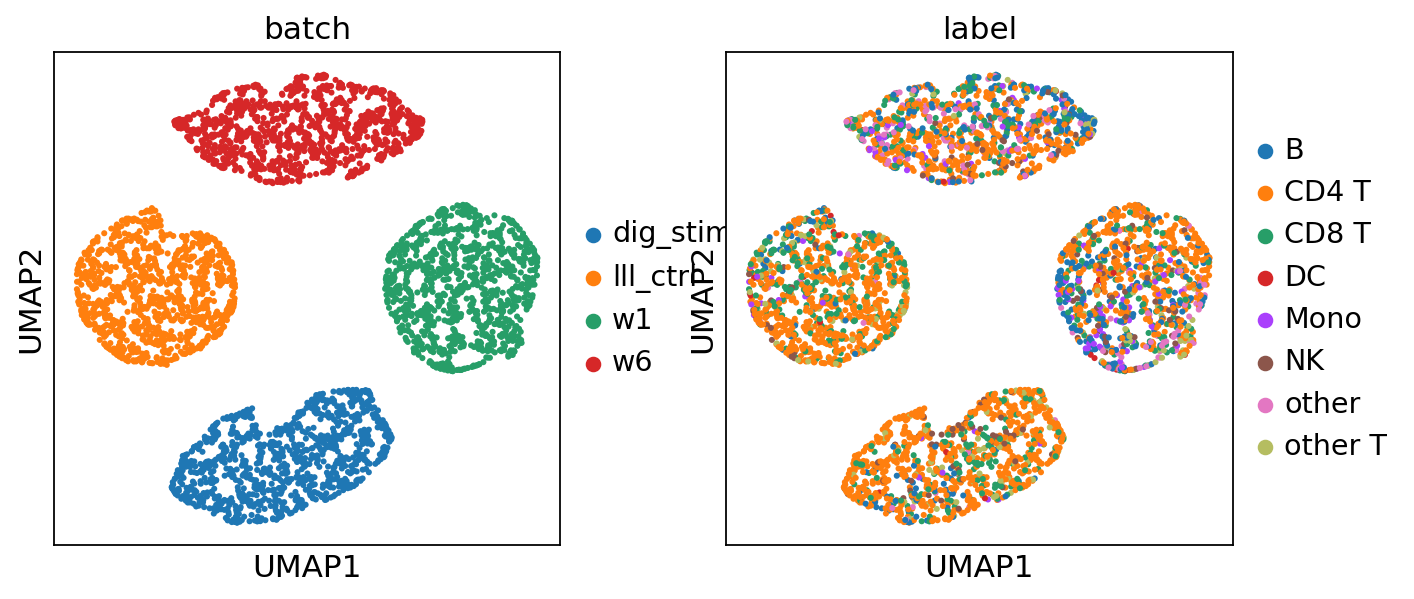
Outputs: Batch-corrected Counts#
[ ]:
batch_corrected_counts = load_predicted('./predict/'+task, model.combs, batch_correct=True)
Only the shared features will be used.
[ ]:
mask = {'rna':[], 'adt':[]}
for i in range(4):
    for m in ['rna', 'adt']:
        try:
            mask[m].append(pd.read_csv('./dataset/'+task+'/data/batch_%d/mask/%s.csv'%(i, m), index_col=0).values)
        except:
            pass
rna_ = pd.DataFrame(batch_corrected_counts['x_bc']['rna'][:, (np.sum(mask['rna'], axis=0)==3)[0]]).T
adt_ = pd.DataFrame(batch_corrected_counts['x_bc']['adt'][:, (np.sum(mask['adt'], axis=0)==3)[0]]).T
atac_ = pd.DataFrame(batch_corrected_counts['x_bc']['atac']).T
rna_.to_csv('./temp_rna.csv', index=True)
adt_.to_csv('./temp_adt.csv', index=True)
atac_.to_csv('./temp_atac.csv', index=True)
Set up the R environment.
[ ]:
from rpy2.robjects.packages import importr
import rpy2.robjects as ro
from rpy2.robjects import pandas2ri
importr('Seurat')
importr('SeuratDisk')
importr('dplyr')
importr('Signac')
Reduction + WNN
[ ]:
ro.r('''
rna <- read.csv('./temp_rna.csv', header=TRUE, row.names=1)
adt <- read.csv('./temp_adt.csv', header=TRUE, row.names=1)
atac <- read.csv('./temp_atac.csv', header=TRUE, row.names=1)
obj <- CreateSeuratObject(counts = rna, assay = "rna")
obj[["adt"]] <- CreateAssayObject(counts = adt)
obj[["atac"]] <- CreateChromatinAssay(counts = atac)
obj <- subset(obj, subset = nCount_atac > 0 & nCount_rna > 0 & nCount_adt > 0)
print(obj)
DefaultAssay(obj) <- 'atac'
obj <-  RunTFIDF(obj) %>%
        FindTopFeatures(min.cutoff = "q25") %>%
        RunSVD(reduction.name = "lsi")
print('finish atac')
DefaultAssay(obj) <- 'rna'
VariableFeatures(obj) <- rownames(obj)
obj <-  NormalizeData(obj) %>%
        # FindVariableFeatures(nfeatures = 2000) %>%
        ScaleData() %>%
        RunPCA(reduction.name = "pca_rna", verbose = F)
print('finish rna')
DefaultAssay(obj) <- 'adt'
VariableFeatures(obj) <- rownames(obj)
obj <-  NormalizeData(obj, normalization.method = "CLR", margin = 2) %>%
        ScaleData() %>%
        RunPCA(reduction.name = "pca_adt", verbose = F)
print('finish adt')
print('WNN ...')
obj <- FindMultiModalNeighbors(obj, list("lsi", "pca_rna", "pca_adt"), list(1:50, 1:50, 1:32))
obj <- RunUMAP(obj, nn.name = "weighted.nn", reduction.name = "umap")
''')
Visualize with scanpy.
[ ]:
# Create an AnnData object with 'X' not being used, so we initialize it with all zeros
adata = sc.AnnData(np.zeros([4000, 1]))
adata.obs['label'] = labels
adata.obs['batch'] = batch_ids
f = ro.r('''
     DimPlot(obj, reduction='umap')
     ''')
adata.obsm['umap'] = pd.DataFrame(f[0]).iloc[:2].T.values
# Shuffle
sc.pp.subsample(adata, fraction=1)
sc.pl.umap(adata, color=['batch', 'label'], ncols=1)
... storing 'label' as categorical
... storing 'batch' as categorical