
Rectangular Integration of RNA+ADT#
In this tutorial, we demonstrate how to integrate a dataset consisting of RNA and ADT data. We will also walk through the inference process and the some of the outputs generated by MIDAS.
Step 1: Downloading the Demo Data#
[ ]:
from scmidas.data import download_data
download_data('wnn_full_3batch', './dataset')
Step 2: Setting Up the Environment#
Before we begin, ensure that the required environment is set up. This includes importing the necessary packages and dependencies.
[ ]:
import os
os.environ['CUDA_VISIBLE_DEVICES']='0'

from scmidas.config import load_config
from scmidas.model import MIDAS
from scmidas.utils import load_predicted
import lightning as L

import pandas as pd
import numpy as np
import scanpy as sc
import matplotlib.pyplot as plt

sc.set_figure_params(figsize=(4, 4))
Step 3: Configuring the Model#
In this step, we configure the model.
[ ]:
configs = load_config() # refer to Tutotrials/Advanced/Development Instructions for details
[ ]:
task = 'wnn_full_3batch'
model = MIDAS.configure_data_from_dir(configs, './dataset/'+task+'/data')
INFO:root:Input data:
         #CELL  #RNA  #ADT  #VALID_RNA  #VALID_ADT
BATCH 0   6378  3617   224        3617         224
BATCH 1   6952  3617   224        3617         224
BATCH 2   8908  3617   224        3617         224
Step 4: Training the Model (~4h)#
After configuring the model, we proceed with training. This step typically takes around 4 hours using a single V100 GPU, depending on your system’s specifications. If you prefer a quicker result, you can set max_epochs=500 for a reasonable outcome, instead of the default max_epochs=2000 for the best result.
[4]:
trainer = L.Trainer(max_epochs=2000)
trainer.fit(model=model)
GPU available: True (cuda), used: True
TPU available: False, using: 0 TPU cores
HPU available: False, using: 0 HPUs
LOCAL_RANK: 0 - CUDA_VISIBLE_DEVICES: [0]

  | Name | Type          | Params | Mode
-----------------------------------------------
0 | net  | VAE           | 8.2 M  | train
1 | dsc  | Discriminator | 39.2 K | train
-----------------------------------------------
8.2 M     Trainable params
0         Non-trainable params
8.2 M     Total params
32.817    Total estimated model params size (MB)
154       Modules in train mode
0         Modules in eval mode
INFO:root:Total number of samples: 22238 from 3 datasets.
INFO:root:Using MultiBatchSampler for data loading.
/root/anaconda3/envs/pl/lib/python3.12/site-packages/torch/utils/data/sampler.py:76: UserWarning: `data_source` argument is not used and will be removed in 2.2.0.You may still have custom implementation that utilizes it.
  warnings.warn(
INFO:root:DataLoader created with batch size 256 and 20 workers.
Epoch 500: 100%|██████████| 105/105 [00:07<00:00, 14.72it/s, v_num=6, loss_/recon_loss_step=2.5e+3, loss_/kld_loss_step=105.0, loss_/consistency_loss_step=20.60, loss/net_step=2.53e+3, loss/dsc_step=97.70, loss_/recon_loss_epoch=2.34e+3, loss_/kld_loss_epoch=105.0, loss_/consistency_loss_epoch=21.40, loss/net_epoch=2.37e+3, loss/dsc_epoch=93.00]
INFO:root:Checkpoint successfully saved to "./saved_models/model_epoch500_20241217-031018.pt".
INFO:root:Checkpoint saved for epoch "500" at "./saved_models/model_epoch500_20241217-031018.pt".
Epoch 1000: 100%|██████████| 105/105 [00:07<00:00, 14.16it/s, v_num=6, loss_/recon_loss_step=2.46e+3, loss_/kld_loss_step=104.0, loss_/consistency_loss_step=18.30, loss/net_step=2.48e+3, loss/dsc_step=93.10, loss_/recon_loss_epoch=2.3e+3, loss_/kld_loss_epoch=102.0, loss_/consistency_loss_epoch=20.60, loss/net_epoch=2.33e+3, loss/dsc_epoch=92.70]
INFO:root:Checkpoint successfully saved to "./saved_models/model_epoch1000_20241217-041043.pt".
INFO:root:Checkpoint saved for epoch "1000" at "./saved_models/model_epoch1000_20241217-041043.pt".
Epoch 1500: 100%|██████████| 105/105 [00:07<00:00, 14.12it/s, v_num=6, loss_/recon_loss_step=2.36e+3, loss_/kld_loss_step=102.0, loss_/consistency_loss_step=18.40, loss/net_step=2.39e+3, loss/dsc_step=93.80, loss_/recon_loss_epoch=2.28e+3, loss_/kld_loss_epoch=101.0, loss_/consistency_loss_epoch=21.00, loss/net_epoch=2.31e+3, loss/dsc_epoch=92.60]
INFO:root:Checkpoint successfully saved to "./saved_models/model_epoch1500_20241217-051155.pt".
INFO:root:Checkpoint saved for epoch "1500" at "./saved_models/model_epoch1500_20241217-051155.pt".
Epoch 1999: 100%|██████████| 105/105 [00:06<00:00, 15.06it/s, v_num=6, loss_/recon_loss_step=2.38e+3, loss_/kld_loss_step=102.0, loss_/consistency_loss_step=18.00, loss/net_step=2.41e+3, loss/dsc_step=94.80, loss_/recon_loss_epoch=2.27e+3, loss_/kld_loss_epoch=101.0, loss_/consistency_loss_epoch=20.70, loss/net_epoch=2.3e+3, loss/dsc_epoch=92.80]
`Trainer.fit` stopped: `max_epochs=2000` reached.
Epoch 1999: 100%|██████████| 105/105 [00:06<00:00, 15.03it/s, v_num=6, loss_/recon_loss_step=2.38e+3, loss_/kld_loss_step=102.0, loss_/consistency_loss_step=18.00, loss/net_step=2.41e+3, loss/dsc_step=94.80, loss_/recon_loss_epoch=2.27e+3, loss_/kld_loss_epoch=101.0, loss_/consistency_loss_epoch=20.70, loss/net_epoch=2.3e+3, loss/dsc_epoch=92.80]
INFO:root:Checkpoint successfully saved to "./saved_models/model_epoch2000_20241217-061343.pt".
INFO:root:Checkpoint saved for epoch "2000" at ./saved_models/model_epoch2000_20241217-061343.pt".
Step 5: Predicting#
Once the model is trained, we can run predict() to obtain various outputs from MIDAS.
[ ]:
model.predict('./predict/'+task,
        joint_latent=True,
        mod_latent=True,
        impute=True,
        batch_correct=True,
        translate=True,
        input=True)
Outputs: Joint Embeddings#
In this step, we explore the various outputs generated by MIDAS. First, we load the cell-type and batch index labels associated with the dataset.
[ ]:
label = []
batch_id = []
for i in ['p1_0', 'p5_0', 'p8_0']:
    label.append(pd.read_csv('./dataset/'+task+'/label/%s.csv'%i, index_col=0).values.flatten())
    batch_id.append([i] * len(label[-1]))
labels = np.concatenate(label)
batch_ids = np.concatenate(batch_id)
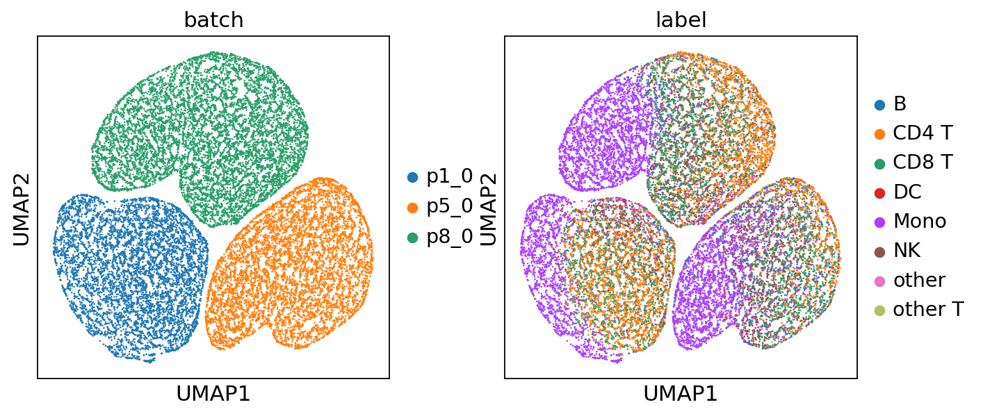
The joint embeddings consist of two components: biological information (c) and technical information (u). To analyze them, we split the embeddings and visualize them separately.
[ ]:
joint_embeddings = load_predicted('./predict/'+task, model.combs, joint_latent=True)

adata_bio = sc.AnnData(joint_embeddings['z']['joint'][:, :model.dim_c])
adata_tech = sc.AnnData(joint_embeddings['z']['joint'][:, model.dim_c:])

adata_bio.obs['batch'] = batch_ids
adata_bio.obs['label'] = labels
adata_tech.obs['batch'] = batch_ids
adata_tech.obs['label'] = labels
# shuffle
sc.pp.subsample(adata_bio, fraction=1)
sc.pp.subsample(adata_tech, fraction=1)
for adata in [adata_bio, adata_tech]:
    sc.pp.neighbors(adata)
    sc.tl.umap(adata)
    sc.pl.umap(adata, color=['batch', 'label'], ncols=2)
INFO:root:Loading predicted variables ...
INFO:root:Loading batch 0: z, joint
100%|██████████| 25/25 [00:00<00:00, 287.99it/s]
INFO:root:Loading batch 1: z, joint
100%|██████████| 28/28 [00:00<00:00, 251.03it/s]
INFO:root:Loading batch 2: z, joint
100%|██████████| 35/35 [00:00<00:00, 243.35it/s]
INFO:root:Converting to numpy ...
INFO:root:Converting batch 0: s, joint
INFO:root:Converting batch 0: z, joint
INFO:root:Converting batch 1: s, joint
INFO:root:Converting batch 1: z, joint
INFO:root:Converting batch 2: s, joint
INFO:root:Converting batch 2: z, joint
... storing 'batch' as categorical
... storing 'label' as categorical

... storing 'batch' as categorical
... storing 'label' as categorical
For quick visualization of the joint embeddings, we provide an API that allows for efficient plotting.
[ ]:
# adata, _ = model.get_emb_umap('../predict/'+task)
Outputs: Modality-specific Embeddings#
MIDAS can generate embeddings for each modality. Here, we check the alignment among modalities by visualizing them with UMAP.
[ ]:
mod_embeddings = load_predicted('./predict/'+task, model.combs, mod_latent=True, group_by='batch')
batch_names = ['p1_0', 'p5_0', 'p8_0']
adata_list = []
for i in range(model.dims_s['joint']):
    for m in model.mods+['joint']:
        if m in mod_embeddings[i]['z']:
            adata = sc.AnnData(mod_embeddings[i]['z'][m][:, :model.dim_c])
            adata.obs['batch'] = batch_names[i]
            adata.obs['modality'] = m
            adata.obs['label'] = label[i]
            adata_list.append(adata)
adata_mod_concat = sc.concat(adata_list)
for i in adata_mod_concat.obs:
    adata_mod_concat.obs[i] = adata_mod_concat.obs[i].astype('category')
sc.pp.neighbors(adata_mod_concat)
# shuffle
sc.pp.subsample(adata_mod_concat, fraction=1)
sc.tl.umap(adata_mod_concat)
[17]:
# setup figure
nrows = len(model.mods) + 1
ncols = model.dims_s['joint']
point_size = 10

fig, ax = plt.subplots(nrows, ncols, figsize=[2 * ncols, 2 * nrows])

# set up the name of modalities and batch
mod_names = model.mods + ['joint']

# iteratively scatter the data
for i, mod in enumerate(mod_names):
    for b in range(model.dims_s['joint']):
        # filter data
        adata = adata_mod_concat[
            (adata_mod_concat.obs['modality'] == mod) &
            (adata_mod_concat.obs['batch'] == batch_names[b])
        ].copy()
        if len(adata):
            sc.pl.umap(adata, color='label', show=False, ax=ax[i, b], s=point_size)
            ax[i, b].get_legend().set_visible(False)
            handles, labels_ = ax[i, b].get_legend_handles_labels()
        ax[i, b].set_xticks([])
        ax[i, b].set_yticks([])
        ax[i, b].set_xlabel('')
        if b==0:
            ax[i, b].set_ylabel(mod.upper())
        else:
            ax[i, b].set_ylabel('')
        if i==0:
            ax[i, b].set_title(batch_names[b])
        else:
            ax[i, b].set_title('')
# create global legend
fig.legend(handles, labels_, loc='center', bbox_to_anchor=(0.5, -0.02), ncol=len(labels_), fontsize=10)

# adjust the figure
plt.tight_layout(rect=[0.1, 0.05, 1, 1])
plt.show()

Outputs: Batch-corrected Counts#
By using the standard noise, we can generate the batch-corrected data. To validate the batch effect in the predicted multi-modalities counts, we use PCA+WNN to gain the joint embeddings for them. First of all, we load the batch-corrected counts.
[ ]:
batch_corrected_counts = load_predicted('./predict/'+task, model.combs, batch_correct=True)
Save the data to CSV files for later use in R.
[ ]:
pd.DataFrame(batch_corrected_counts['x_bc']['rna']).T.to_csv('temp_rna.csv', index=True)
pd.DataFrame(batch_corrected_counts['x_bc']['adt']).T.to_csv('temp_adt.csv', index=True)
Set up the R environment.
[ ]:
from rpy2.robjects.packages import importr
import rpy2.robjects as ro
importr('Seurat')
importr('SeuratDisk')
importr('dplyr')
importr('Signac')
PCA+WNN
[ ]:
ro.r('''
rna <- read.csv('./temp_rna.csv', header=TRUE, row.names=1)
adt <- read.csv('./temp_adt.csv', header=TRUE, row.names=1)
obj <- CreateSeuratObject(counts = rna, assay = "rna")
obj[["adt"]] <- CreateAssayObject(counts = adt)
obj <- subset(obj, subset = nCount_rna > 0 & nCount_adt > 0)
print(obj)
DefaultAssay(obj) <- 'rna'
VariableFeatures(obj) <- rownames(obj)
obj <-  NormalizeData(obj) %>%
        # FindVariableFeatures(nfeatures = 2000) %>%
        ScaleData() %>%
        RunPCA(reduction.name = "pca_rna", verbose = F)
print('finish rna')
DefaultAssay(obj) <- 'adt'
VariableFeatures(obj) <- rownames(obj)
obj <-  NormalizeData(obj, normalization.method = "CLR", margin = 2) %>%
        ScaleData() %>%
        RunPCA(reduction.name = "pca_adt", verbose = F)
print('finish adt')
print('WNN ...')
obj <- FindMultiModalNeighbors(obj, list("pca_rna", "pca_adt"), list(1:32, 1:32))
obj <- RunUMAP(obj, nn.name = "weighted.nn", reduction.name = "umap")
''')
[ ]:
# Create an AnnData object with 'X' not being used, so we initialize it with all zeros
adata = sc.AnnData(np.zeros([len(batch_corrected_counts['x_bc']['rna']), 1]))
adata.obs['label'] = labels
adata.obs['batch'] = batch_ids
f = ro.r('''DimPlot(obj, reduction='umap')''')
adata.obsm['umap'] = pd.DataFrame(f[0]).iloc[:2].T.values
# shuffle
sc.pp.subsample(adata, fraction=1)
sc.pl.umap(adata, color=['batch', 'label'], ncols=1)
... storing 'label' as categorical
... storing 'batch' as categorical

Similarly, we load the raw counts and visualize the UMAP using the same procedure.
[ ]:
inputs = load_predicted('../predict/'+task, model.combs, input=True, group_by='modality')
[17]:
pd.DataFrame(inputs['x']['rna']).T.to_csv('temp_rna.csv', index=True)
pd.DataFrame(inputs['x']['adt']).T.to_csv('temp_adt.csv', index=True)
[ ]:
ro.r('''
rna <- read.csv('./temp_rna.csv', header=TRUE, row.names=1)
adt <- read.csv('./temp_adt.csv', header=TRUE, row.names=1)
obj <- CreateSeuratObject(counts = rna, assay = "rna")
obj[["adt"]] <- CreateAssayObject(counts = adt)
obj <- subset(obj, subset = nCount_rna > 0 & nCount_adt > 0)
print(obj)
DefaultAssay(obj) <- 'rna'
VariableFeatures(obj) <- rownames(obj)
obj <-  NormalizeData(obj) %>%
        # FindVariableFeatures(nfeatures = 2000) %>%
        ScaleData() %>%
        RunPCA(reduction.name = "pca_rna", verbose = F)
print('finish rna')
DefaultAssay(obj) <- 'adt'
VariableFeatures(obj) <- rownames(obj)
obj <-  NormalizeData(obj, normalization.method = "CLR", margin = 2) %>%
        ScaleData() %>%
        RunPCA(reduction.name = "pca_adt", verbose = F)
print('finish adt')
print('WNN ...')
obj <- FindMultiModalNeighbors(obj, list("pca_rna", "pca_adt"), list(1:32, 1:32))
obj <- RunUMAP(obj, nn.name = "weighted.nn", reduction.name = "umap")
''')
[19]:
adata = sc.AnnData(np.zeros([len(inputs['x']['rna']), 1]))
adata.obs['label'] = labels
adata.obs['batch'] = batch_ids
f = ro.r('''
     DimPlot(obj, reduction='umap')
     ''')
adata.obsm['umap'] = pd.DataFrame(f[0]).iloc[:2].T.values
# shuffle
sc.pp.subsample(adata, fraction=1)
sc.pl.umap(adata, color=['batch', 'label'], ncols=1)
... storing 'label' as categorical
... storing 'batch' as categorical
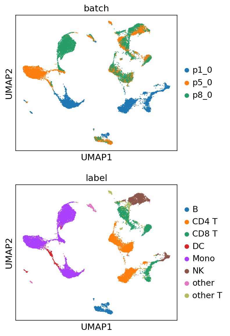
For the raw data, prominent batch effects are observed, where clusters of cells are segregated based on batches. For the MIDAS batch-corrected counts, these batch effects are effectively removed, leading to well-integrated clusters.